Multiverse integration

Comet includes multiverse integration methods based on the weighting schemes introduced in:

Cantone, G. G., & Tomaselli, V. (2025). Characterisation and calibration of multiversal methods.

Advances in Data Analysis and Classification, 19(4), 989-1021. https://doi.org/10.1007/s11634-024-00610-9

For illustration and validation purposes, we use the “unidentified multiverse” example from the paper, which was introduced in a previous paper by Del Giudice and Gangestad (2021). https://doi.org/10.6084/m9.figshare.12089736

from comet.multiverse import Multiverse

forking_paths = {
    "X1": [0, 1],
    "X2": [0, 1],
    "X3": [0, 1],
    "X4": [0, 1],
    "ANTE": [0, 1],
    "MEDI": [0, 1],
    "COLL": [0, 1],
    "CONF": [0, 1],
}

def analysis_template():
    import comet
    import statsmodels.formula.api as smf

    data = comet.utils.load_example("cantone")

    # Build composite predictor
    data["pred"] = 0.0
    if {{X1}}:
        data["pred"] += data["BM1"]
    if {{X2}}:
        data["pred"] += data["BM2"]
    if {{X3}}:
        data["pred"] += data["BM3"]
    if {{X4}}:
        data["pred"] += data["BM4"]

    # Build covariates
    cov = ""
    if {{ANTE}}:
        cov += " + genotype"
    if {{MEDI}}:
        cov += " + pain"
    if {{COLL}}:
        cov += " + fatigue"
    if {{CONF}}:
        cov += " + age"

    # Regression model
    formula = "depression ~ pred" + cov
    fit_res = smf.ols(formula=formula, data=data).fit()

    beta_raw = float(fit_res.params["pred"])
    sd_y = float(data["depression"].std())
    sd_x = float(data["pred"].std())
    beta_std = beta_raw * (sd_x / sd_y)

    out = {
        "formula": formula,
        "beta": float(beta_std),
        "beta_raw": float(beta_raw),
        "p_value": float(fit_res.pvalues["pred"]),
    }

    comet.utils.save_universe_results(out)

config = {
    "remove": [
        [{"X1": 0}, {"X2": 0}, {"X3": 0}, {"X4": 0}],
    ]
}

mverse = Multiverse(name="example_mv_integration")
mverse.create(analysis_template, forking_paths, config)
mverse.summary()
mverse.run(parallel=16)

Removed 16 out of 256 universes:

	Universe	Decision 1	Value 1	Decision 2	Value 2	Decision 3	Value 3	Decision 4	Value 4	Decision 5	Value 5	Decision 6	Value 6	Decision 7	Value 7	Decision 8	Value 8
0	Universe_1	X1	0	X2	0	X3	0	X4	1	ANTE	0	MEDI	0	COLL	0	CONF	0
1	Universe_2	X1	0	X2	0	X3	0	X4	1	ANTE	0	MEDI	0	COLL	0	CONF	1
2	Universe_3	X1	0	X2	0	X3	0	X4	1	ANTE	0	MEDI	0	COLL	1	CONF	0
3	Universe_4	X1	0	X2	0	X3	0	X4	1	ANTE	0	MEDI	0	COLL	1	CONF	1
4	Universe_5	X1	0	X2	0	X3	0	X4	1	ANTE	0	MEDI	1	COLL	0	CONF	0
...	...	...	...	...	...	...	...	...	...	...	...	...	...	...	...	...	...
235	Universe_236	X1	1	X2	1	X3	1	X4	1	ANTE	1	MEDI	0	COLL	1	CONF	1
236	Universe_237	X1	1	X2	1	X3	1	X4	1	ANTE	1	MEDI	1	COLL	0	CONF	0
237	Universe_238	X1	1	X2	1	X3	1	X4	1	ANTE	1	MEDI	1	COLL	0	CONF	1
238	Universe_239	X1	1	X2	1	X3	1	X4	1	ANTE	1	MEDI	1	COLL	1	CONF	0
239	Universe_240	X1	1	X2	1	X3	1	X4	1	ANTE	1	MEDI	1	COLL	1	CONF	1

240 rows × 17 columns

Starting multiverse analysis for all universes...

The multiverse analysis completed without any errors.

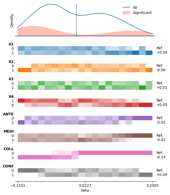
We visualise the multiverse results:

mverse.multiverse_plot(measure="beta", n_bins=20, sig_col="p_value", baseline=0, figsize=(7,9))

Comet currently contains two methods for integrating over the multiverse:

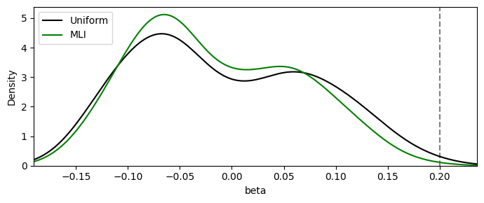
uniform

• All universes are weighted equally (the estimate is just the plain mean/median across universes). This corresponds to the density function as plotted in the multiverse plot above.

mli (Maximum Local Influence)

• Each universe is compared with its nearest neighbours (specifications differing by a single decision). Universes whose estimate barely changes when one decision is flipped are weighted more, down-weighting results that hinge on a single arbitrary choice.

As an example, we can use the .integrate() method to simply get an integrated measure over all universes. For example, using uniform weighting and mean aggregation:

estimate, weights = mverse.integrate(measure="beta", method="uniform", type="mean")
print(f"Mean beta: {estimate:.4f}")

Mean beta: -0.0066

We can also use the compare_integration and plot_integration convenience functions to get a summary for both integration methods.

table, weights = mverse.compare_integration(measure="beta", true_value=0.2)
table

	Scheme	median	mean	gini_w	err_median	err_mean
0	Uniform	-0.0210	-0.0066	0.000	0.221	0.207
1	MLI	-0.0328	-0.0144	0.243	0.233	0.214

The columns are, for each weighting scheme:

• median / mean: the integrated estimate (weighted median/mean of beta)

• gini_w: how concentrated the weights are (0 = all equal, → 1 = dominated by a few universes).

If true_value is passed, additional err_* columns give the absolute error of each estimate against it. Usually, this is not available in real multiverses, but we can include it here as we have the ground truth from the simulation.

mverse.plot_integration(measure="beta", weights=weights, true_value=0.2)