Visualising a multiverse

As an example, we inspect the famous “Female hurricanes are deadlier than male hurricanes” multiverse from Simonsohn et al. (2020). The implementation of this multiverse is implemented in the Hurricane multiverse (non-neuroimaging) example below.

We start by loading the multiverse from memory and print the forking paths as a table:

from comet import multiverse

mverse = multiverse.load_multiverse("example_mv_hurricane")
mverse.summary()

	Universe	Decision 1	Value 1	Decision 2	Value 2	Decision 3	Value 3	Decision 4	Value 4	Decision 5	Value 5	Decision 6	Value 6	Decision 7	Value 7
0	Universe_1	death_outliers	2	damage_outliers	3	femininity_rating	fem_likert	damage_functional	ln	effect_type	femininity * damages	year_interaction	NaN	model	log_linear
1	Universe_2	death_outliers	2	damage_outliers	3	femininity_rating	fem_likert	damage_functional	ln	effect_type	femininity * damages	year_interaction	NaN	model	neg_binomial
2	Universe_3	death_outliers	2	damage_outliers	3	femininity_rating	fem_likert	damage_functional	ln	effect_type	femininity * damages	year_interaction	+ post1979:damages	model	log_linear
3	Universe_4	death_outliers	2	damage_outliers	3	femininity_rating	fem_likert	damage_functional	ln	effect_type	femininity * damages	year_interaction	+ post1979:damages	model	neg_binomial
4	Universe_5	death_outliers	2	damage_outliers	3	femininity_rating	fem_likert	damage_functional	ln	effect_type	femininity * damages	year_interaction	+ year:damages	model	log_linear
...	...	...	...	...	...	...	...	...	...	...	...	...	...	...	...
1723	Universe_1724	death_outliers	0	damage_outliers	0	femininity_rating	fem_binary	damage_functional	linear	effect_type	femininity + damages + z3	year_interaction	NaN	model	neg_binomial
1724	Universe_1725	death_outliers	0	damage_outliers	0	femininity_rating	fem_binary	damage_functional	linear	effect_type	femininity + damages + z3	year_interaction	+ post1979:damages	model	log_linear
1725	Universe_1726	death_outliers	0	damage_outliers	0	femininity_rating	fem_binary	damage_functional	linear	effect_type	femininity + damages + z3	year_interaction	+ post1979:damages	model	neg_binomial
1726	Universe_1727	death_outliers	0	damage_outliers	0	femininity_rating	fem_binary	damage_functional	linear	effect_type	femininity + damages + z3	year_interaction	+ year:damages	model	log_linear
1727	Universe_1728	death_outliers	0	damage_outliers	0	femininity_rating	fem_binary	damage_functional	linear	effect_type	femininity + damages + z3	year_interaction	+ year:damages	model	neg_binomial

1728 rows × 15 columns

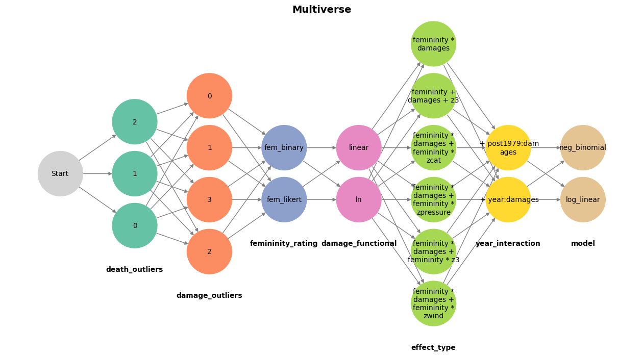
We can visualise the structure any linear multiverse as a feed-forward network:

mverse.visualize(figsize=(16, 8), text_size=10, node_size=4000)

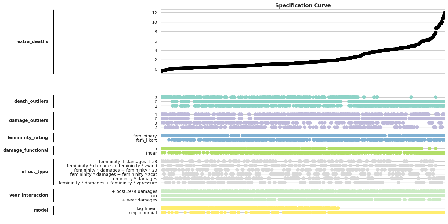
The results of a multiverse can be visualised with two main functions, namely a specification curve and a multiverse plot.

A traditional specification curve plots the results of each multiverse against the individual specification. This is often useful, but does not scale well with large multiverses like the present one:

mverse.specification_curve("extra_deaths", figsize=(12,9), height_ratio=(1,2), line_pad=0.05)

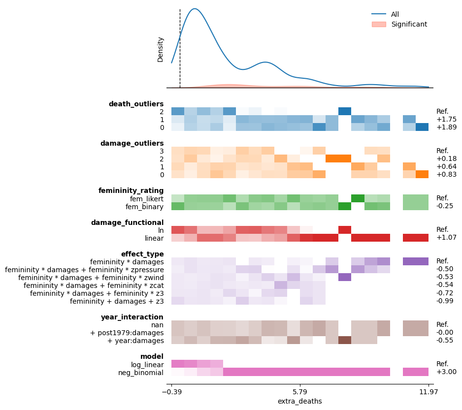
A more modern alternative is a multiverse plot, which visualises the results as a density function and groups the specifications into bins (Krähmer & Young, 2026). Here it becomes easily visible how most effects are close to 0 and not significant.

Krähmer, D., & Young, C. (2026). Visualizing vastness: Graphical methods for multiverse analysis. PLOS One, 21(2), e0339452. https://doi.org/10.1371/journal.pone.0339452

mverse.multiverse_plot(measure="extra_deaths", n_bins=20, sig_col="p_val", baseline=0, figsize=(7,10))