Graphical user interface quickstart
The GUI allows you to load and explore the following types of data:
fMRIprep-processed datasets
NIFTI files (
.nii,.nii.gz)CIFTI files (
.dtseries.nii)Time series data in multiple formats (
.txt,.csv,.tsv,.npy,.mat)
Downloading data
Single NIfTI file
verbose=1 if you would like to see the download progress.)[1]:
from nilearn import datasets

save_dir = "."
adhd_data = datasets.fetch_adhd(data_dir=save_dir, n_subjects=1)
[fetch_adhd] Dataset found in adhd
BIDS Dataset
As a secod option, you can fetch fMRIprep-processed data from the Engaging in word recognition elicits highly specific modulations in visual cortex dataset (ds004489) on OpenNeuro:
pip install datalad-installer
datalad-installer git-annex -m datalad/packages
pip install datalad
You can then install the dataset in the current working directory and download a single BOLD + confounds file by typing:
datalad install https://github.com/OpenNeuroDatasets/ds004489.git
cd ds004489
datalad get derivatives/sub-114/ses-1/func/sub-114_ses-1_task-catLoc_run-1_space-T1w_desc-preproc_bold.nii.gz
datalad get derivatives/sub-114/ses-1/func/sub-114_ses-1_task-catLoc_run-1_desc-confounds_timeseries.tsv
Starting the GUI
comet-gui in the terminal.comet, this will looks something like this:(comet) user@pc:~$ comet-gui
As a result, you should be greeted with the data tab of the graphical user interface.
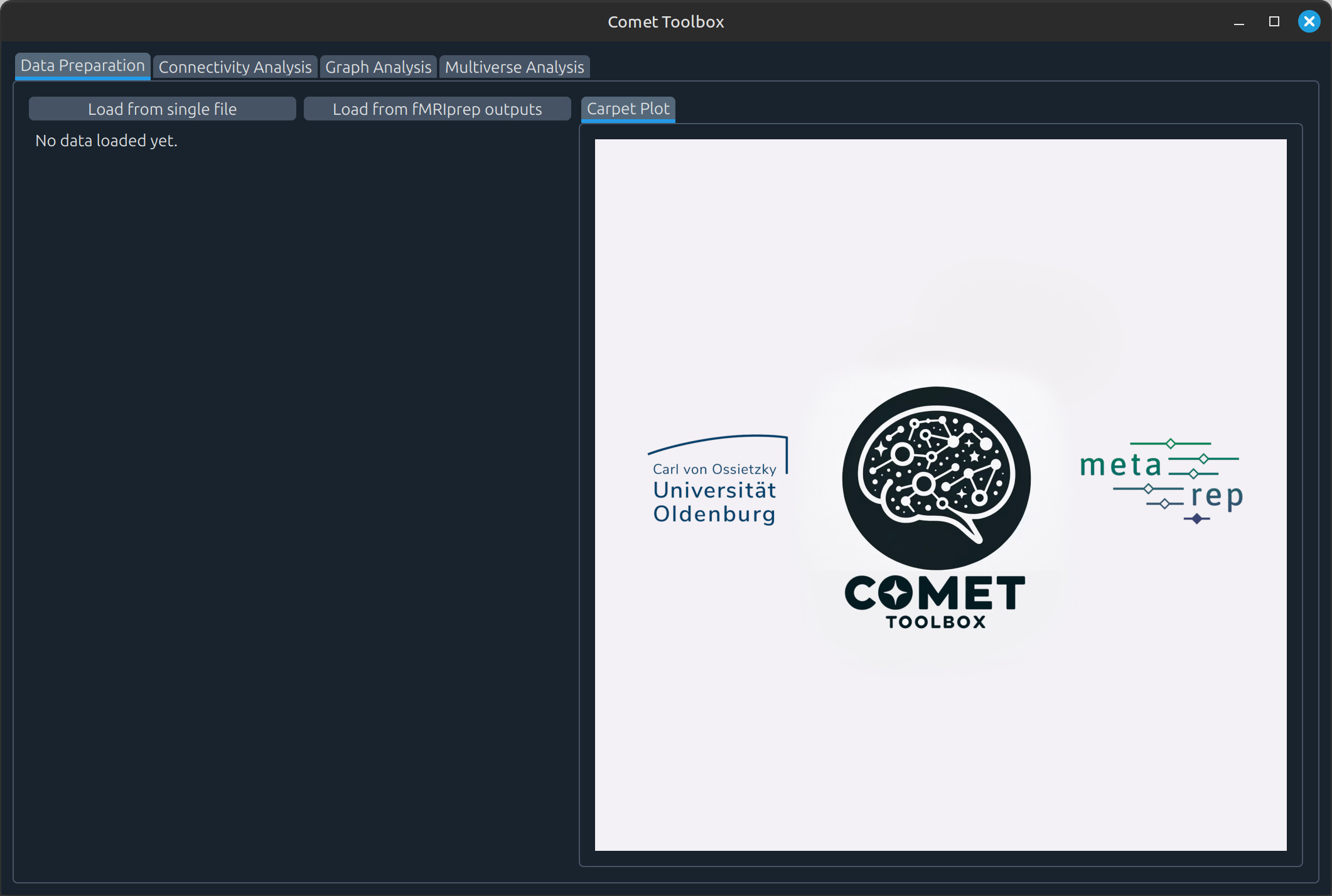
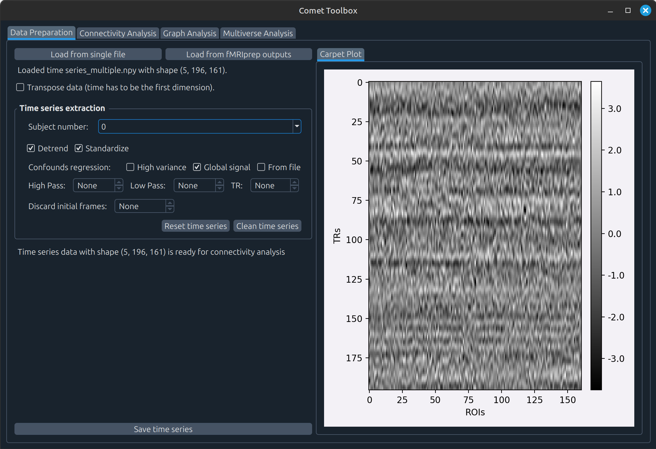
Data preparation
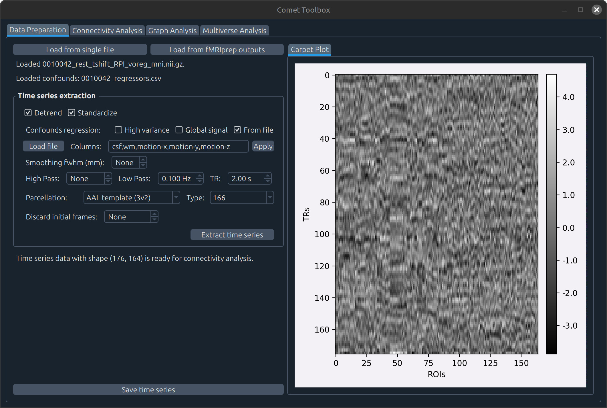
Using a single NIFTI file
adhd/data/0010042/0010042_rest_tshift_RPI_voreg_mni.nii.gz.A panel will appear with several preprocessing options, such as:
Detrending and standardising the data (enabled by default)
Temporal filtering (requires the TR to be specified)
Selecting a parcellation scheme
Discarding initial frames (non-stationary volumes are also detected automatically)
…
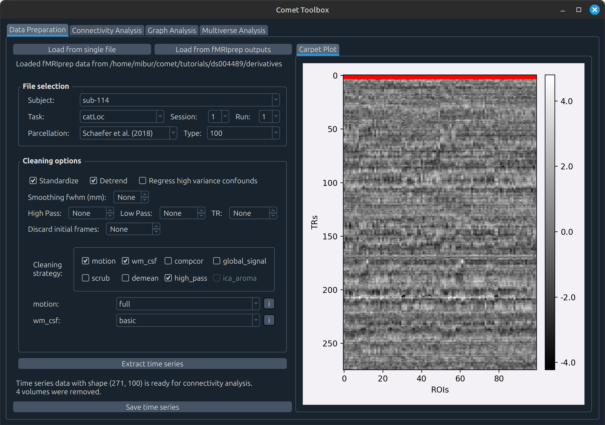
Using fMRIprep-processed data
Click Load from fMRIprep outputs and open the ds004489/derivatives folder.
Once the dataset layout is loaded, select:
Subject:
sub114Task:
catLocSession:
1Run:
1
Note: Although the full dataset structure is initialised, only the data for this specific participant and run was downloaded above.
For example, in the screenshot below we selected motion, wm_csf, and high_pass
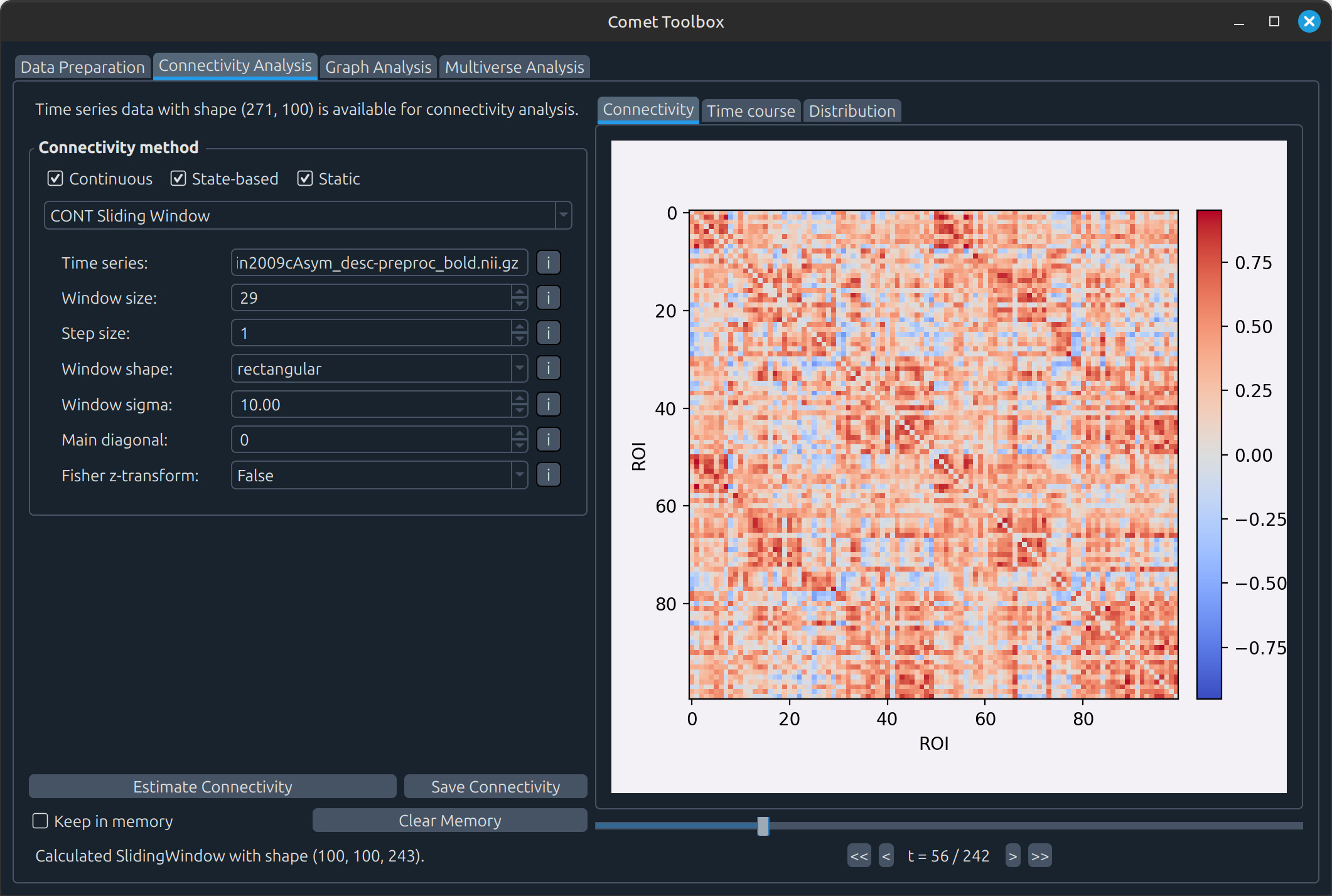
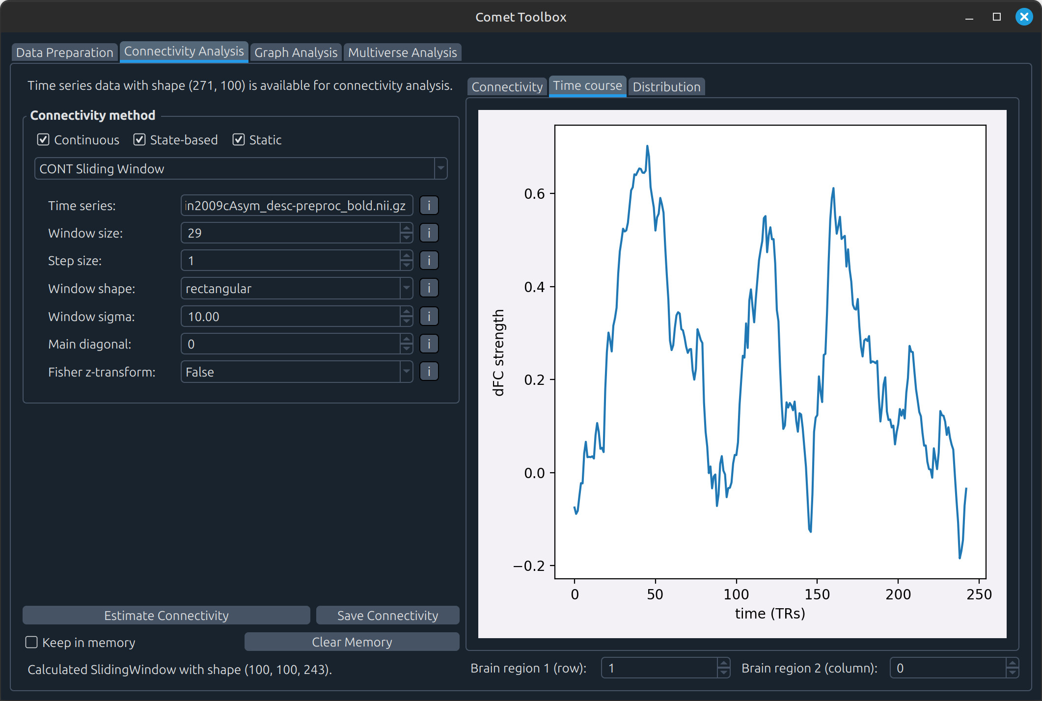
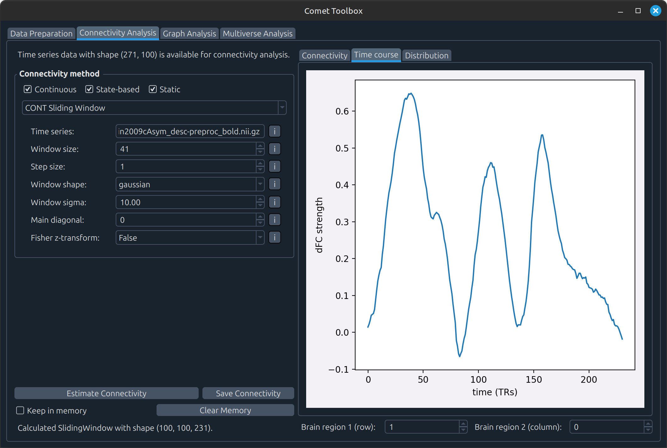
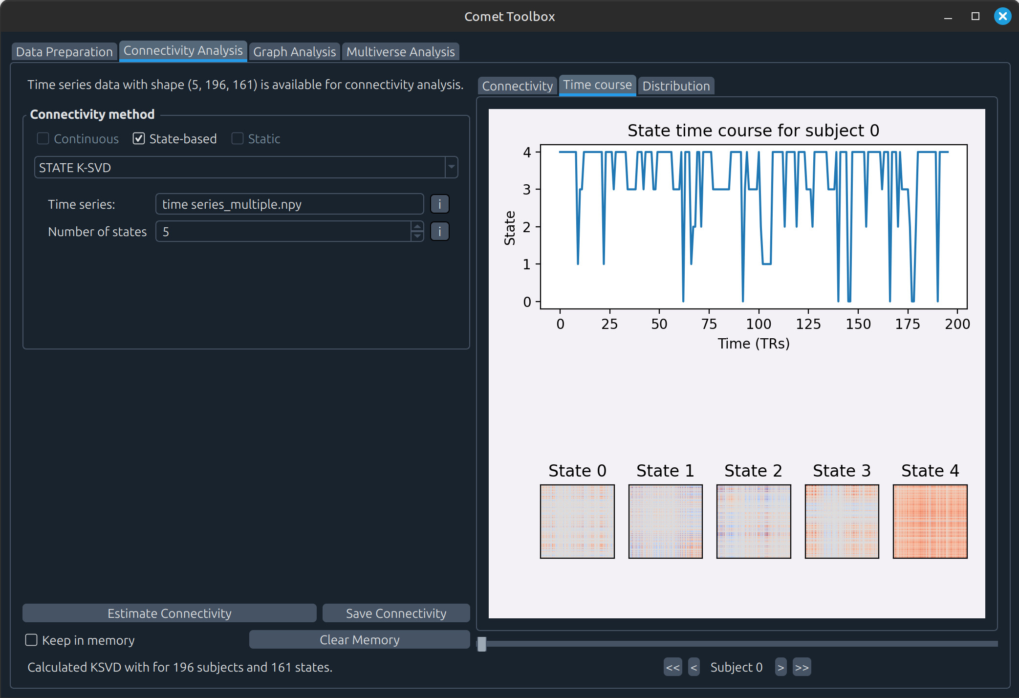
Connectivity analysis
State-based analysis
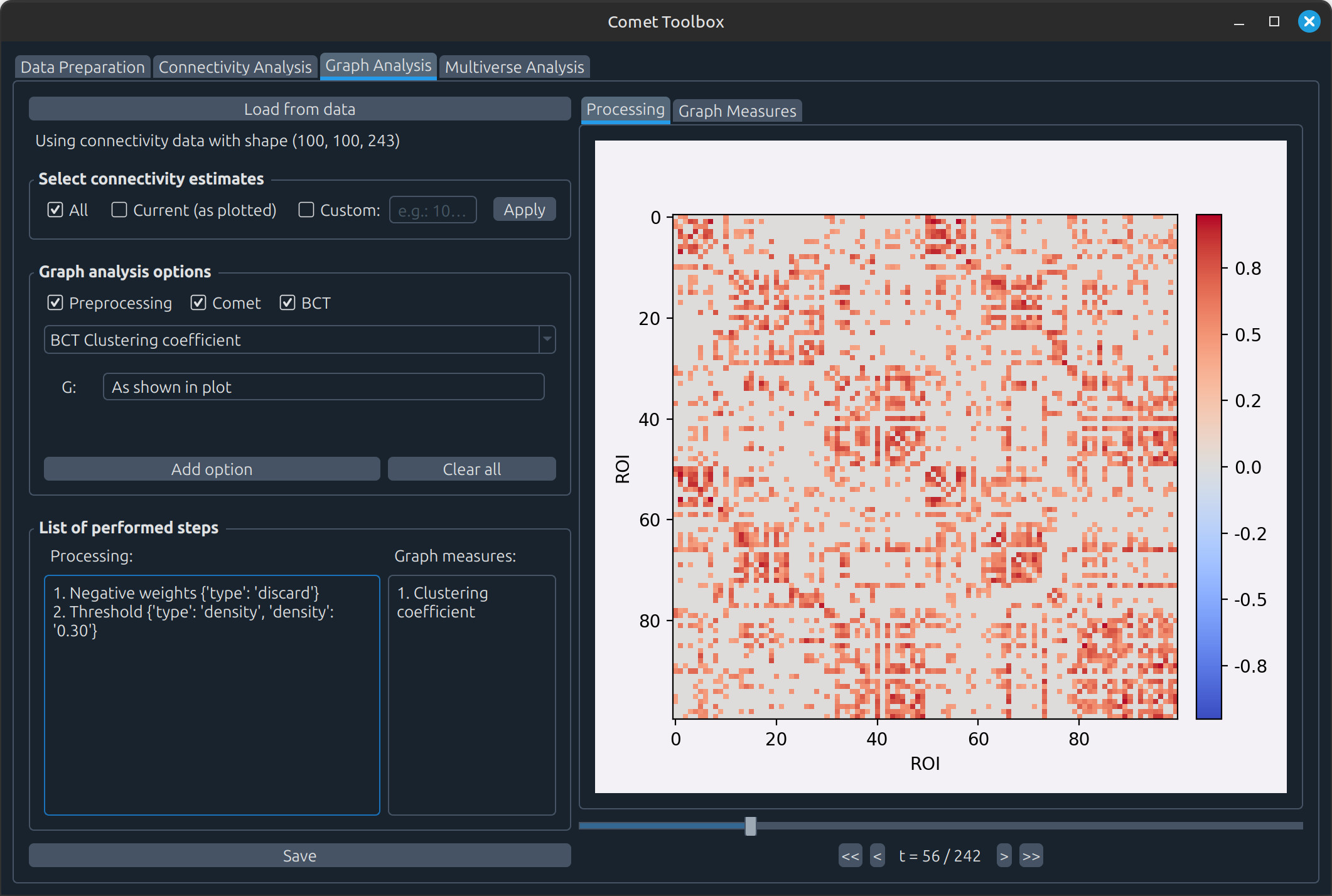
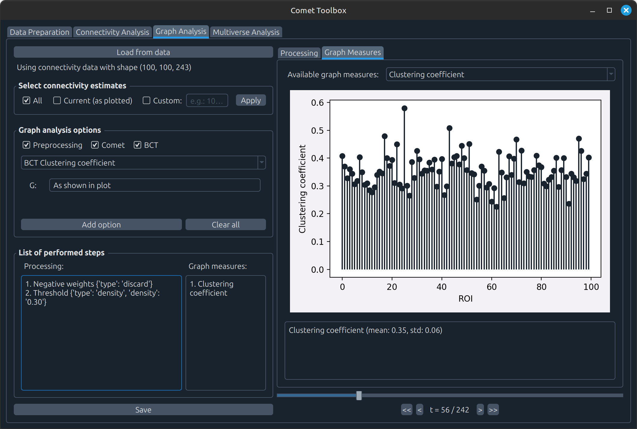
Graph analysis
The typical workflow is as follows:
Apply processing steps to the connectivity matrices, such as handling negative values or applying thresholding. Example: In the screenshots below, negative values were removed and matrices were thresholded to 40% density before computing the clustering coefficient.
Estimate graph measures, which are then visualised in the Graph Measures tab.
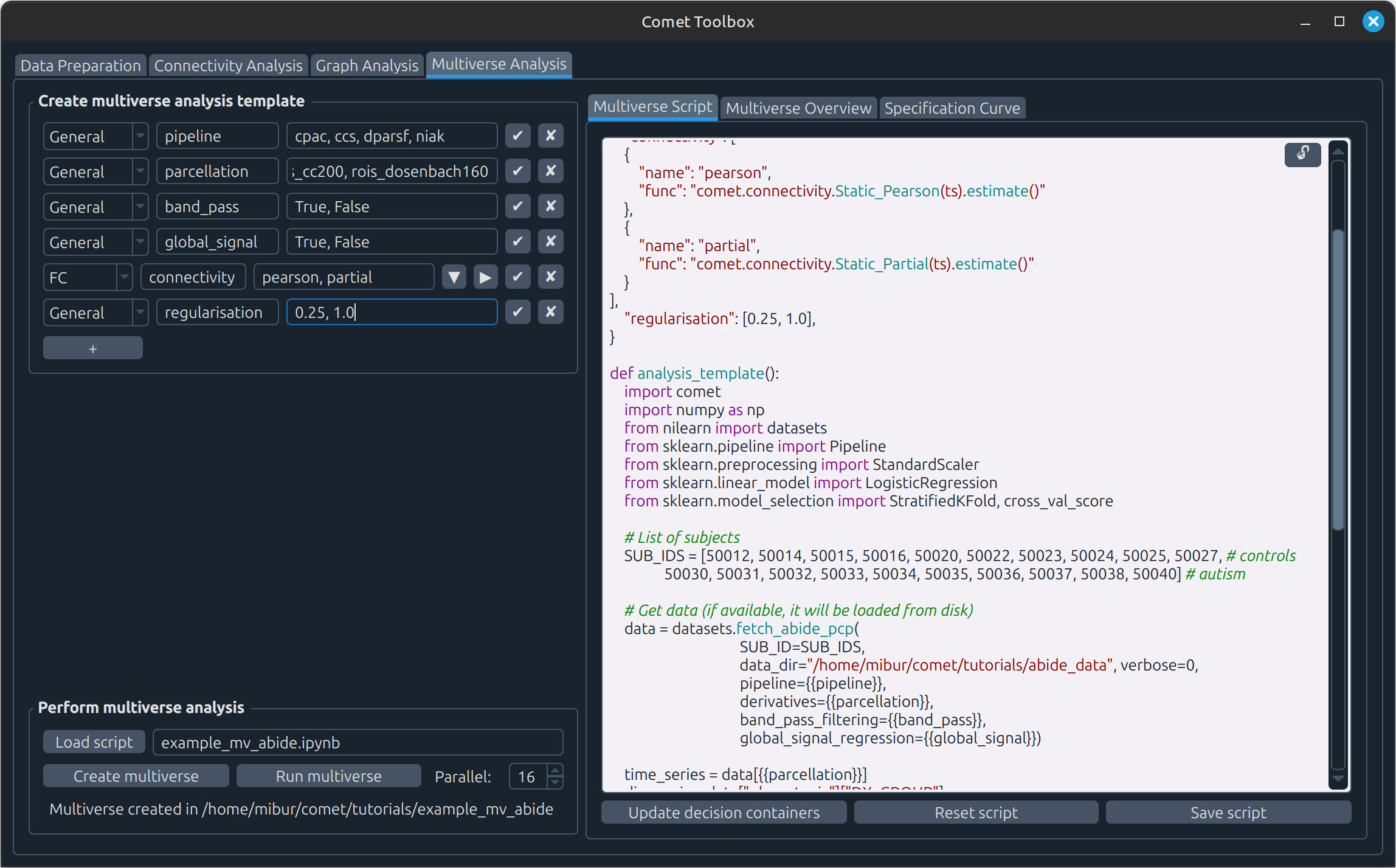
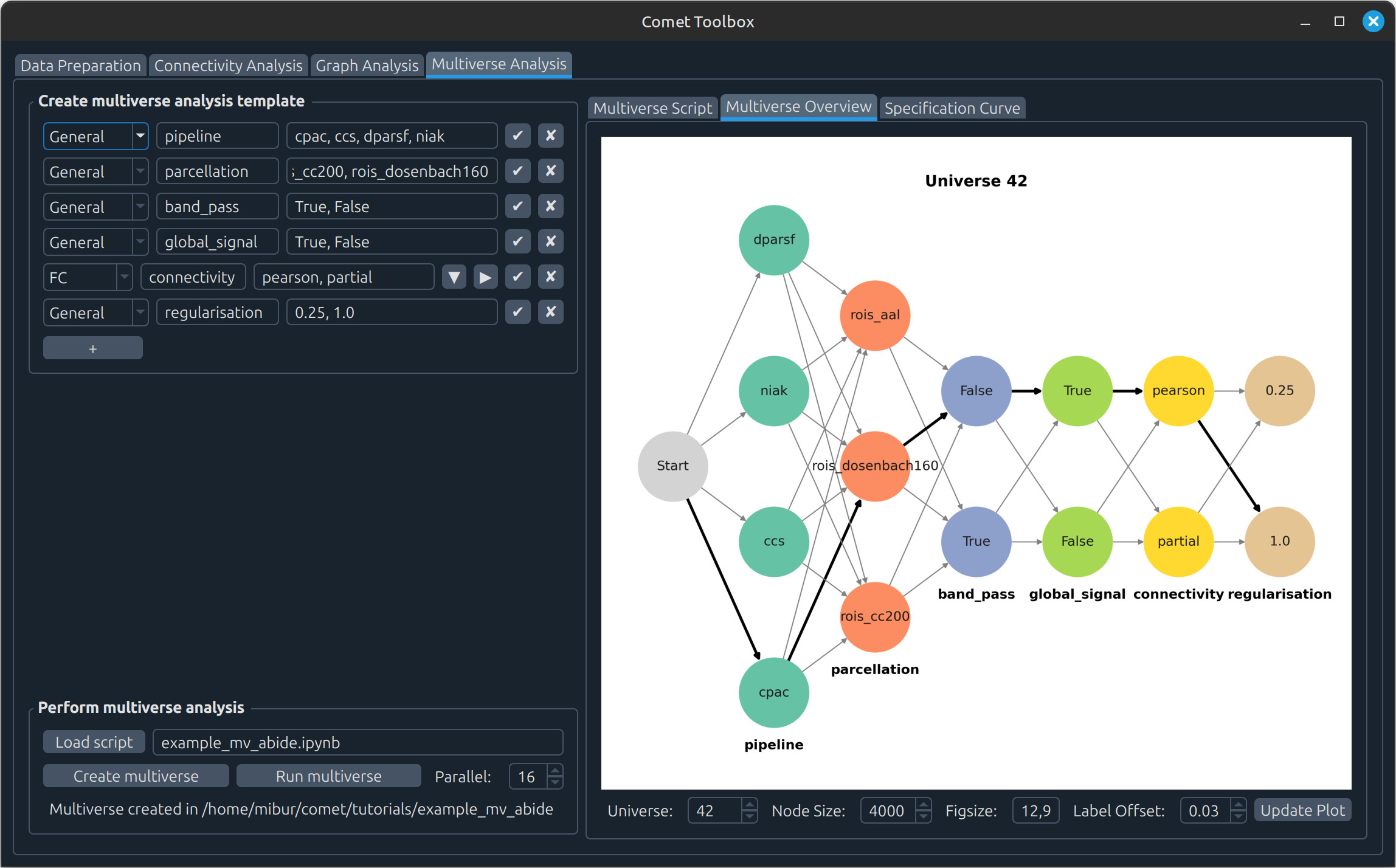
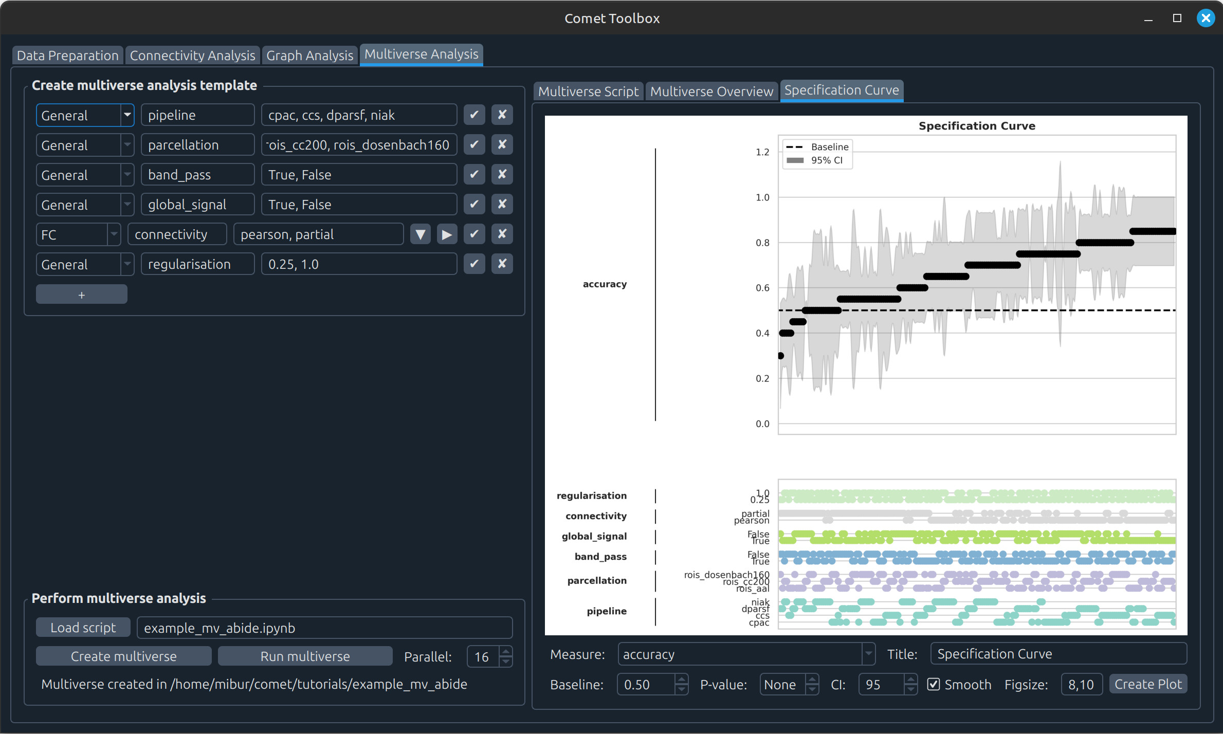
Multiverse analysis
Click Create multiverse to open a file dialog and choose where the multiverse analysis folder should be created.
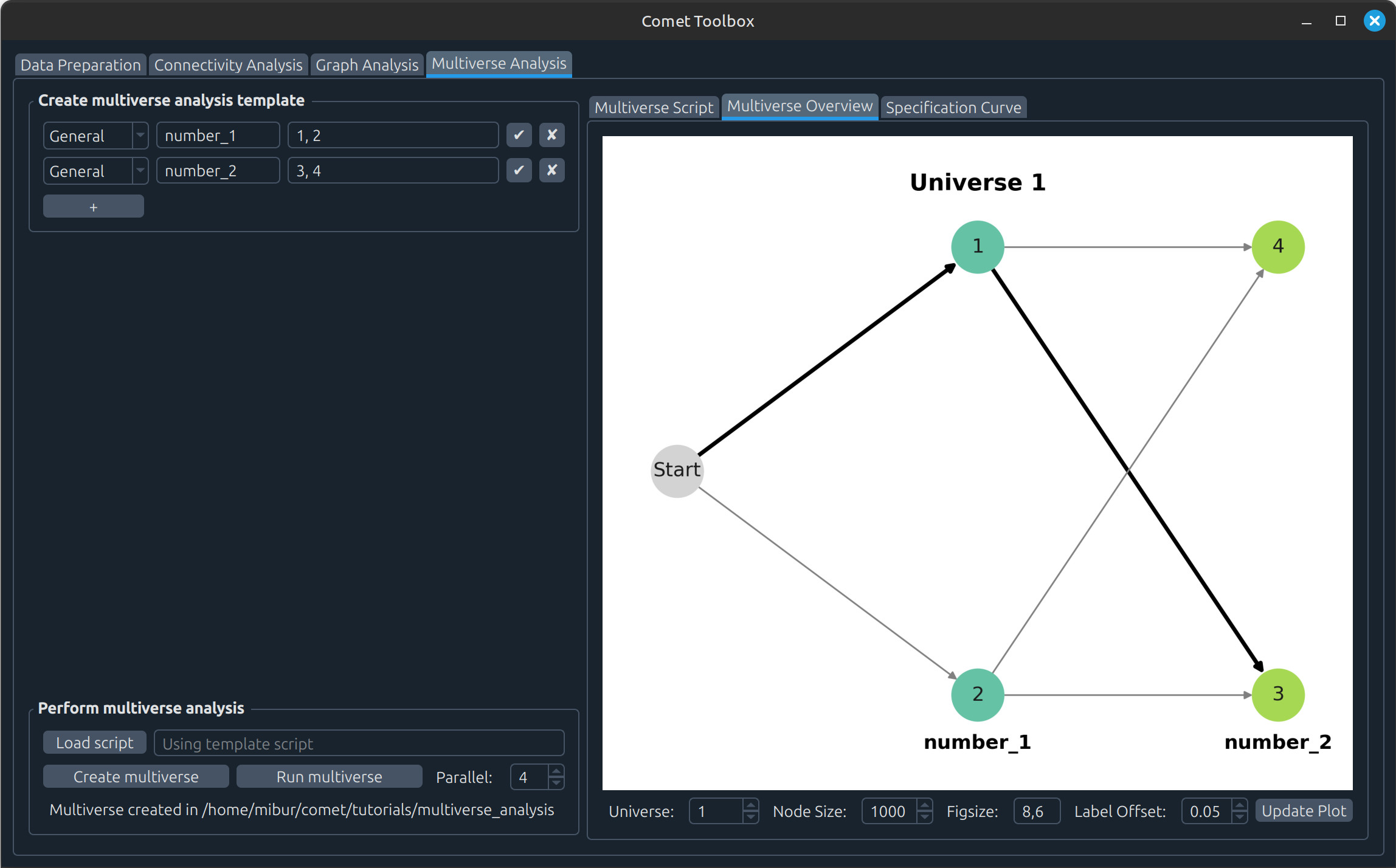
Click Run multiverse to execute the analysis. Results will then appear in the Multiverse Overview and Specification Curve tabs.
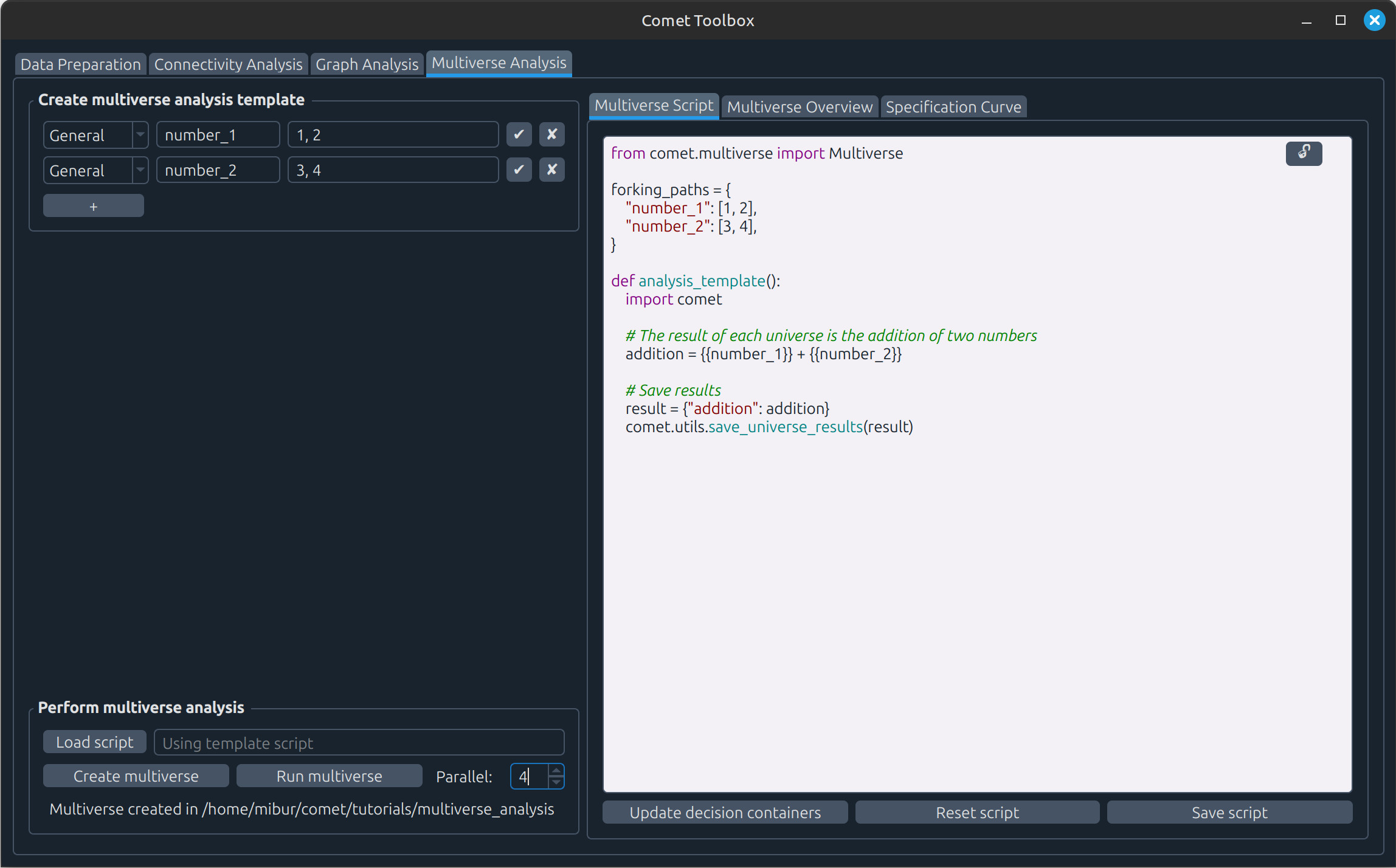
You can also modify the example:
For instance, add the number
5to thenumber_2decision and confirm with the checkmark button.If you don’t mind overwriting previous results, you can skip creating a new multiverse and simply press Run multiverse again to update the analysis.
Running a previously implemented multiverse analysis
For example, the autism classification workflow can be loaded from tutorials/example_mv_abide.ipynb and explored in the GUI. Before creating and running the multiverse, make sure you have previously downloaded the data as described in tutorials/example_mv_abide.ipynb and provide an absolute path to it (as well as a a subset of subjects to speed up the calculation):
SUB_IDS = [50012, 50014, 50015, 50016, 50020, 50022, 50023, 50024, 50025, 50027, # controls
           50030, 50031, 50032, 50033, 50034, 50035, 50036, 50037, 50038, 50040] # autism

# Get data (if available, it will be loaded from disk)
data = datasets.fetch_abide_pcp(SUB_ID=SUB_IDs,
                                data_dir="<PATH_TO_DATA>",
                                verbose=0,
                                pipeline={{pipeline}},
                                derivatives={{parcellation}},
                                band_pass_filtering={{band_pass}},
                                global_signal_regression={{global_signal}})