Graph measures

This script showcases how to use some graph measures included in the comet toolbox.

import numpy as np
from nilearn import datasets
from matplotlib import pyplot as plt
from comet import graph

# Get preprocessed time series data from the ABIDE dataset
subjects = [50008, 50010, 50012, 50014]
data = datasets.fetch_abide_pcp(SUB_ID=subjects, pipeline='cpac', band_pass_filtering=True, derivatives="rois_dosenbach160")

[fetch_abide_pcp] Dataset found in /home/mibur/nilearn_data/ABIDE_pcp

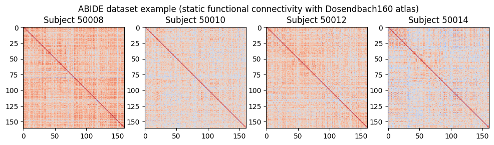
Calculate and plot static functional connectivity:

fig, ax = plt.subplots(1,4, figsize=(12,3))
fig.suptitle('ABIDE dataset example (static functional connectivity with Dosendbach160 atlas)')

fc = []
for sub in range(len(subjects)):
    ts = data.rois_dosenbach160[sub]
    corr = np.corrcoef(ts.T)
    fc.append(corr)
    ax[sub].imshow(corr, cmap='coolwarm', vmin=-1, vmax=1)
    ax[sub].set_title('Subject %d' % subjects[sub])

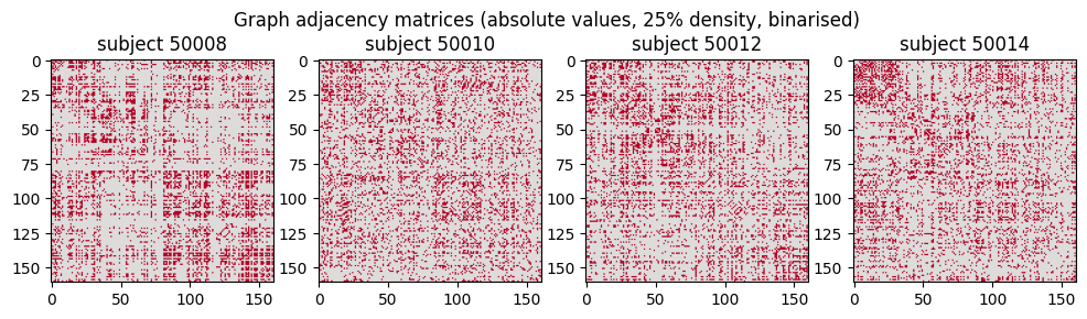
Graph construction and plotting of the resulting adjacency matrices:

fig, ax = plt.subplots(1,4, figsize=(12,3))
fig.suptitle('Graph adjacency matrices (absolute values, 25% density, binarised)')

G = []
for i, sub in enumerate(subjects):
    g = graph.handle_negative_weights(fc[i], type="absolute")
    g = graph.threshold(g, type="density", density=0.2)
    g = graph.binarise(g)
    ax[i].imshow(g, cmap='coolwarm', vmin=-1, vmax=1)
    ax[i].set_title(f"subject {sub}")
    G.append(g)

Calculate small-world sigma:

for i, sub in enumerate(subjects):
    swp1 = graph.small_world_propensity(G[i])[0]
    print(f"Subject {sub} small-world propensity: {swp1:.2f}")

/home/mibur/repositories/comet/src/comet/graph.py:555: UserWarning: The graph is not fully connected; infinite path lengths were set to NaN.
  warnings.warn("The graph is not fully connected; infinite path lengths were set to NaN.")

Subject 50008 small-world propensity: 0.72
Subject 50010 small-world propensity: 0.52
Subject 50012 small-world propensity: 0.65
Subject 50014 small-world propensity: 0.60

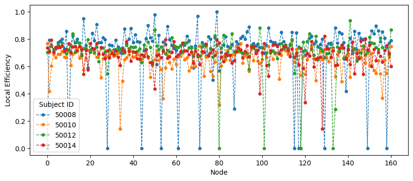
Calculate local efficiency:

eff = []
for i, sub in enumerate(subjects):
    eff.append(graph.efficiency(G[i], local=True))

eff = np.asarray(eff).T

plt.figure(figsize=(10,4))
plt.plot(eff, label=subjects, marker='o', markersize=4, linestyle='--', linewidth=1)
plt.xlabel('Node')
plt.ylabel('Local Efficiency')
plt.legend(title="Subject ID");