State-based dFC

Currently, Comet includes five explicit state-based dFC methods as published in:

Mohammad Torabi, Georgios D Mitsis, Jean-Baptiste Poline, On the variability of dynamic functional connectivityassessment methods, GigaScience, Volume 13, 2024, giae009, https://doi.org/10.1093/gigascience/giae009.

• Sliding Window Clustering

• Coactivation Patterns

• Continuous Hidden Markov Model

• Discrete Hidden Markov Model

• Windowless (K-SVD) Model

State-based connectivity analysis usually uses data from multiple subjects, so we start by getting some pre-processed time series data from the ABIDE dataset which we put in a list (a single 3D numpy array would also be fine):

import numpy as np
from nilearn import datasets
from comet import connectivity, utils

subjects = ["50008", "50010", "50012", "50014", "50020"]
data = datasets.fetch_abide_pcp(SUB_ID=subjects, pipeline='cpac', band_pass_filtering=True, derivatives="rois_dosenbach160")
ts = data.rois_dosenbach160 # list of 2D time series data

print("Num subjects:",len(ts))
print("TS shape:", ts[0].shape)

[fetch_abide_pcp] Dataset found in /home/mibur/nilearn_data/ABIDE_pcp

Num subjects: 5
TS shape: (196, 161)

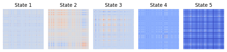
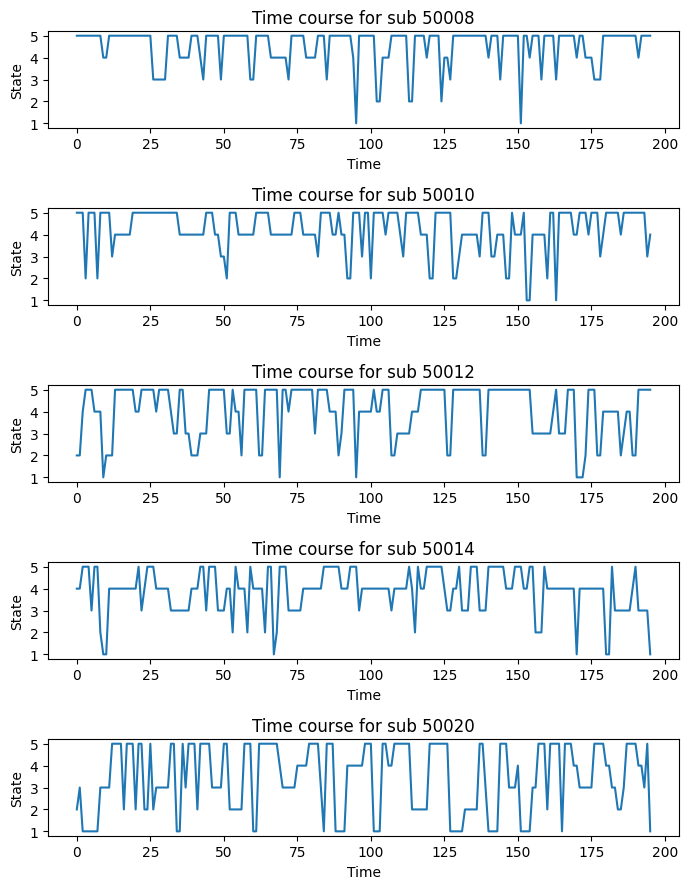
We can then calculate state-based functional connectivity with any of the methods, e.g. KSVD:

ksvd = connectivity.KSVD(ts, n_states=5)
state_tc, states = ksvd.estimate()

# Plot states and state time courses
fig1, ax1 = utils.state_plots(states=states, figsize=(8,2))
fig2, ax2 = utils.state_plots(state_tc=state_tc, figsize=(7,9), sub_ids=subjects)

Or Coactivation Patterns:

cap = connectivity.CoactivationPatterns(ts, n_states=5)
state_tc, states = cap.estimate()

CAP: 100%|██████████| 5/5 [00:00<00:00, 17.76it/s]

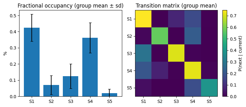
Further summary statistics can also be calculated and plotted as follows:

summary = utils.summarise_state_tc(state_tc)

# You can print the summary statistics
dwell_mean = summary["fractional_occupancy"].mean(axis=0)
dwell_std = summary["fractional_occupancy"].std(axis=0)
trans_mean = summary["transitions"].mean(axis=0)

print("Fractional occupancy (mean ± sd):\n", np.round(dwell_mean, 3), "±", np.round(dwell_std, 3))
print("Mean transition matrix:\n",  np.round(trans_mean, 3))

# Or you can plot them
summary = utils.summarise_state_tc(state_tc)
fig3, ax3 = utils.state_plots(summary=summary, figsize=(8,3.5))

Fractional occupancy (mean ± sd):
 [0.423 0.07  0.126 0.361 0.019] ± [0.084 0.059 0.076 0.093 0.027]
Mean transition matrix:
 [[0.748 0.    0.078 0.17  0.004]
 [0.012 0.571 0.    0.218 0.   ]
 [0.284 0.    0.708 0.008 0.   ]
 [0.201 0.067 0.004 0.718 0.01 ]
 [0.029 0.    0.    0.181 0.39 ]]