Preparing CIFTI data for connectivity analysis

CIFTI data refers to surface-level data as e.g. used in the Human Connectome Project (HCP).

For this tutorial, you will need to create a BALSA account and then download the data for a single subject first, e.g. by selecting:

ConnectomeDB -> HCP-Young Adult 2025 -> Subject group: Single subject -> Resting State fMRI 3T Preprocessed Recommended

Note: this download will require approximately 10GB of disk space.

Once downloaded and unpacked, you can load a single CIFTI file. In this case, one resting-state run from the HCP contains 1200 time points and 91282 vertices:

import nibabel as nib

dtseries = nib.load("100307/MNINonLinear/Results/rfMRI_REST1_LR/rfMRI_REST1_LR_Atlas_MSMAll_hp2000_clean_rclean_tclean.dtseries.nii")
print(dtseries.shape)

(1200, 91282)

As the data is already cleaned, we do not need to perform further denoising. For parcellation, we can simply use thee cifti.parcellate() function which offers many commonly used atlasses.

For example, the following code cell will perform parcellation with Schaefer 200 cortical + 54 subcortical ROIs and then estimates dynamic functional connectivity with the sliding window correlation method:

from comet import cifti, connectivity

ts = cifti.parcellate(dtseries, atlas="schaefer", resolution=200, subcortical="S4")

sw = connectivity.SlidingWindow(ts, windowsize=51, shape="gaussian")
dfc = sw.estimate()
print(dfc.shape)

/home/mibur/miniconda3/envs/comet-test/lib/python3.13/site-packages/tqdm_joblib/__init__.py:4: TqdmExperimentalWarning: Using `tqdm.autonotebook.tqdm` in notebook mode. Use `tqdm.tqdm` instead to force console mode (e.g. in jupyter console)
  from tqdm.autonotebook import tqdm

(254, 254, 1150)

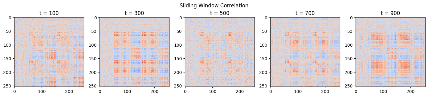
Finally, we can plot the resulting estimates at different time points:

from matplotlib import pyplot as plt

centers = sw.centers() # time points (center of the window) for each estimate

fig, ax = plt.subplots(1, 5, figsize=(14, 3))
fig.suptitle("Sliding Window Correlation")

for i in range(5):
    t = i*200 + 75
    ax[i].set_title(f"t = {centers[t]}")
    ax[i].imshow(dfc[:,:,t], cmap="coolwarm", vmin=-1, vmax=1)

plt.tight_layout()